Chapter 2 R basic data manipulations
2.1 Introduction to R Syntax
R is a powerful programming language designed specifically for statistical computing and data analysis. Let’s explore its fundamental concepts.
2.1.1 Variables and Data Types
Before diving into coding, it’s essential to understand the basic data types in R. Think of variables as containers that store different types of information. R has three main types of data that you’ll use frequently:
# Numeric (integers and decimals)
# Numbers can be whole (integers) or have decimal points
my_number <- 42.5
print(my_number)
## [1] 42.5# Character (text strings)
# Any text data must be enclosed in quotes
my_text <- "Hello R Markdown!"
print(my_text)## [1] "Hello R Markdown!"# Logical (boolean values)
# TRUE/FALSE values are useful for conditional operations
my_logical <- TRUE
print(my_logical)## [1] TRUEThe <- symbol is the assignment operator in R. While you can use =, <- is preferred in the R community. Let’s practice creating meaningful variables:
# Create and assign variables
age <- 25        # Numeric
name <- "Alice"  # Character
is_student <- TRUE  # Logical

# Display our variables
print(age)
## [1] 25## [1] "Alice"## [1] TRUE# Check variable types using class()
# This is useful to confirm what type of data you're working with
class(age)## [1] "numeric"## [1] "character"## [1] "logical"2.1.2 Basic Operations
R can perform various arithmetic operations just like a calculator. These operations are fundamental to data analysis: addition, subtraction, multiplication, division
# Basic arithmetic operations are straightforward
addition <- 10 + 5       # Adding numbers
subtraction <- 10 - 5    # Subtracting numbers
multiplication <- 10 * 5 # Multiplying numbers
division <- 10 / 5       # Dividing numbers

# Display results
print(addition)
## [1] 15## [1] 5## [1] 50## [1] 2# More complex mathematical operations
power <- 2^3 # Exponentiation (2 to the power of 3)
square_root <- sqrt(16) # Square root function
print(power)## [1] 8## [1] 4Logical operations are crucial for data filtering and conditional statements:
# Comparison operators return TRUE or FALSE
equals <- 5 == 5        # Equality comparison
greater_than <- 10 > 5  # Greater than comparison
less_than <- 3 < 7     # Less than comparison

# Logical operators combine TRUE/FALSE values
and_operator <- TRUE & TRUE    # Both conditions must be TRUE
or_operator <- TRUE | FALSE    # At least one condition must be TRUE

# Print results
print(equals)
## [1] TRUE## [1] TRUE## [1] TRUE## [1] TRUE## [1] TRUE2.2 Objects in R
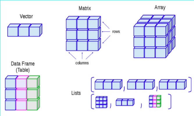
2.2.1 Working with Vectors
Vectors are one of the most basic data structures in R. Think of them as a collection of elements of the same type, like a list of numbers or strings:
# Creating vectors using the combine function c()
numeric_vector <- c(1, 2, 3, 4, 5)           # Vector of numbers
character_vector <- c("apple", "banana", "cherry", "avocado", "mango")  # Vector of strings
logical_vector <- c(TRUE, FALSE, TRUE)       # Vector of logical values

# Display vectors
print(numeric_vector)
## [1] 1 2 3 4 5## [1] "apple" "banana" "cherry" "avocado" "mango"## [1] TRUE FALSE TRUE# Vector operations - R can perform operations on entire vectors at once
# This is called vectorization and is very efficient
print(length(numeric_vector)) # length of the vector## [1] 5## [1] 2 4 6 8 10# Accessing elements using indexing
# R uses 1-based indexing (first element is at position 1, not 0)
first_element <- numeric_vector[1] # Get first element
selected_elements <- numeric_vector[c(1, 3, 5)] # Get specific elements
print(first_element)## [1] 1## [1] 1 3 52.2.2 Creating Sequences
R provides several convenient ways to create sequences of numbers, which is particularly useful for data analysis and plotting:
# Using seq() for more control over sequence generation
sequence1 <- seq(1, 10)          # Basic sequence from 1 to 10
sequence2 <- seq(0, 20, by = 2)  # Even numbers from 0 to 20

# Using : operator for simple sequences
sequence3 <- 1:10                # Another way to create sequence from 1 to 10

# Using rep() to repeat values
repeated <- rep(5, times = 3)    # Repeat the number 5 three times

print(sequence1)
## [1] 1 2 3 4 5 6 7 8 9 10## [1] 0 2 4 6 8 10 12 14 16 18 20## [1] 1 2 3 4 5 6 7 8 9 10## [1] 5 5 52.3 Exercise 1
Understanding Data Types
Create three variables and assign them values of different data types:
- A numeric variable representing your height in centimeters.
- A character variable storing your favorite fruit.
- A logical variable indicating whether you like R programming.
Then, print each variable and use class() to check its data type.
Basic Arithmetic Operations
Perform the following calculations and store the results in variables:
- Multiply 15 by 3.
- Subtract 7 from 100.
- Compute the square root of 64.
- Raise 3 to the power of 4.
Print all results.
Vector Manipulation
Create a numeric vector containing the numbers 2, 4, 6, 8, 10. Multiply all elements of the vector by 3. Extract the second and fourth elements of the vector.
Create a character vector with three country names of your choice. Multiply it by 3.
Creating Sequences
- Create a sequence of numbers from 5 to 50 with a step size of 5.
- Generate a sequence of odd numbers from 1 to 15 using seq().
- Use rep() to create a vector that repeats the number 7 five times.
2.3.1 Working with Data Frames
Data frames are the most common way to work with structured data in R. They’re similar to Excel spreadsheets or database tables:
# Create a simple data frame
# Each column can have a different data type
students_df <- data.frame(
  name = c("Monelson", "Noemie", "Alphonse", "Aichatou", "Laurene", "Anonkoua"),    # Character column
  age = c(25, 20, 23, 22, 22, 26),                    # Numeric column
  note = c(10, 15, 13, 15, 16.5, 9),                 # Numeric column
  is_graduate = c(FALSE, TRUE, TRUE, TRUE, T, F)      # Logical column
)

# Display the data frame
print(students_df)
## name age note is_graduate
## 1 Monelson 25 10.0 FALSE
## 2 Noemie 20 15.0 TRUE
## 3 Alphonse 23 13.0 TRUE
## 4 Aichatou 22 15.0 TRUE
## 5 Laurene 22 16.5 TRUE
## 6 Anonkoua 26 9.0 FALSE## [1] 25 20 23 22 22 26## name age note is_graduate
## 5 Laurene 22 16.5 TRUE# Add a new column - must match the number of rows
students_df$height <- c(175, 168, 182, 150, 160, 155)
print(students_df)## name age note is_graduate height
## 1 Monelson 25 10.0 FALSE 175
## 2 Noemie 20 15.0 TRUE 168
## 3 Alphonse 23 13.0 TRUE 182
## 4 Aichatou 22 15.0 TRUE 150
## 5 Laurene 22 16.5 TRUE 160
## 6 Anonkoua 26 9.0 FALSE 1552.4 Importing an Manipulating data in R
2.4.1 Importing data
# Installing and Loading the Required Package

## First, install and load the `medicaldata` package to access the `covid_testing` dataset.


# Install the package (only needs to be done once)
## install.packages("medicaldata")

# Load the package into the R session
library("medicaldata")

# Load the COVID-19 testing dataset from the medicaldata package
covid <- medicaldata::covid_testing

# Display the first few rows of the dataset
head(covid)
## subject_id fake_first_name fake_last_name gender pan_day test_id
## 1 1412 jhezane westerling female 4 covid
## 2 533 penny targaryen female 7 covid
## 3 9134 grunt rivers male 7 covid
## 4 8518 melisandre swyft female 8 covid
## 5 8967 rolley karstark male 8 covid
## 6 11048 megga karstark female 8 covid
## clinic_name result demo_group age drive_thru_ind ct_result orderset
## 1 inpatient ward a negative patient 0.0 0 45 0
## 2 clinical lab negative patient 0.0 1 45 0
## 3 clinical lab negative patient 0.8 1 45 1
## 4 clinical lab negative patient 0.8 1 45 1
## 5 emergency dept negative patient 0.8 0 45 1
## 6 oncology day hosp negative patient 0.8 0 45 0
## payor_group patient_class col_rec_tat rec_ver_tat
## 1 government inpatient 1.4 5.2
## 2 commercial not applicable 2.3 5.8
## 3 <NA> <NA> 7.3 4.7
## 4 <NA> <NA> 5.8 5.0
## 5 government emergency 1.2 6.4
## 6 commercial recurring outpatient 1.4 7.0## [1] "subject_id" "fake_first_name" "fake_last_name" "gender"
## [5] "pan_day" "test_id" "clinic_name" "result"
## [9] "demo_group" "age" "drive_thru_ind" "ct_result"
## [13] "orderset" "payor_group" "patient_class" "col_rec_tat"
## [17] "rec_ver_tat"## [1] 17## [1] 155242.4.2 Data Frame Manipulation
Data frames support powerful operations for data analysis:
# Filter data based on conditions
high_gpa <- students_df[students_df$gpa > 3.5, ]  # Select rows where GPA > 3.5
print(high_gpa)
## [1] name age note is_graduate height
## <0 lignes> (ou 'row.names' de longueur nulle)# Sort data using order()
sorted_by_age <- students_df[order(students_df$age), ] # Sort by age
print(sorted_by_age)## name age note is_graduate height
## 2 Noemie 20 15.0 TRUE 168
## 4 Aichatou 22 15.0 TRUE 150
## 5 Laurene 22 16.5 TRUE 160
## 3 Alphonse 23 13.0 TRUE 182
## 1 Monelson 25 10.0 FALSE 175
## 6 Anonkoua 26 9.0 FALSE 155## [1] 20 22 22 23 25 262.5 Exercise 2
Import the “blood_storage” database from the package medicaldata.
Log-transform the variable age in data and save the result as age.log.
Square all values in PVol (Prostate volume) and save the result as PVol.squared within the dataset.
Check whether the AA (African American race) is of class factor (0 = “non‐African-American”; 1 = “African American”).
Filter out the records for which (PreopPSA >= 10) and (Recurrence == 0).
In the fifth and sixth rows of the data, change the value of Age to NA (missing).
Remove the variables from the dataset: AA,FamHx,OrganConfined.
Remember that R is case-sensitive and very particular about syntax. Pay attention to brackets, commas, and quotation marks. The best way to learn is by experimenting with the code and modifying it to see what happens!