Chapter 3 Data Wrangling and basic statistics
3.1 1. Introduction to dplyr
The dplyr package is a powerful tool in R for data manipulation. It provides functions for filtering, selecting, arranging, summarizing, and mutating data in an easy and readable way. The %>% (pipe operator) is commonly used to link functions together.
# Install and load necessary packages
#install.packages("dplyr")
#install.packages("medicaldata")

library(dplyr)
##
## Attachement du package : 'dplyr'## Les objets suivants sont masqués depuis 'package:stats':
##
## filter, lag## Les objets suivants sont masqués depuis 'package:base':
##
## intersect, setdiff, setequal, union## [1] "%>%" "across" "add_count"
## [4] "add_count_" "add_row" "add_rownames"
## [7] "add_tally" "add_tally_" "all_equal"
## [10] "all_of" "all_vars" "anti_join"
## [13] "any_of" "any_vars" "arrange"
## [16] "arrange_" "arrange_all" "arrange_at"
## [19] "arrange_if" "as.tbl" "as_data_frame"
## [22] "as_label" "as_tibble" "auto_copy"
## [25] "band_instruments" "band_instruments2" "band_members"
## [28] "bench_tbls" "between" "bind_cols"
## [31] "bind_rows" "c_across" "case_match"
## [34] "case_when" "changes" "check_dbplyr"
## [37] "coalesce" "collapse" "collect"
## [40] "combine" "common_by" "compare_tbls"
## [43] "compare_tbls2" "compute" "consecutive_id"
## [46] "contains" "copy_to" "count"
## [49] "count_" "cross_join" "cumall"
## [52] "cumany" "cume_dist" "cummean"
## [55] "cur_column" "cur_data" "cur_data_all"
## [58] "cur_group" "cur_group_id" "cur_group_rows"
## [61] "current_vars" "data_frame" "db_analyze"
## [64] "db_begin" "db_commit" "db_create_index"
## [67] "db_create_indexes" "db_create_table" "db_data_type"
## [70] "db_desc" "db_drop_table" "db_explain"
## [73] "db_has_table" "db_insert_into" "db_list_tables"
## [76] "db_query_fields" "db_query_rows" "db_rollback"
## [79] "db_save_query" "db_write_table" "dense_rank"
## [82] "desc" "dim_desc" "distinct"
## [85] "distinct_" "distinct_all" "distinct_at"
## [88] "distinct_if" "distinct_prepare" "do"
## [91] "do_" "dplyr_col_modify" "dplyr_reconstruct"
## [94] "dplyr_row_slice" "ends_with" "enexpr"
## [97] "enexprs" "enquo" "enquos"
## [100] "ensym" "ensyms" "eval_tbls"
## [103] "eval_tbls2" "everything" "explain"
## [106] "expr" "failwith" "filter"
## [109] "filter_" "filter_all" "filter_at"
## [112] "filter_if" "first" "full_join"
## [115] "funs" "funs_" "glimpse"
## [118] "group_by" "group_by_" "group_by_all"
## [121] "group_by_at" "group_by_drop_default" "group_by_if"
## [124] "group_by_prepare" "group_cols" "group_data"
## [127] "group_indices" "group_indices_" "group_keys"
## [130] "group_map" "group_modify" "group_nest"
## [133] "group_rows" "group_size" "group_split"
## [136] "group_trim" "group_vars" "group_walk"
## [139] "grouped_df" "groups" "id"
## [142] "ident" "if_all" "if_any"
## [145] "if_else" "inner_join" "intersect"
## [148] "is.grouped_df" "is.src" "is.tbl"
## [151] "is_grouped_df" "join_by" "lag"
## [154] "last" "last_col" "last_dplyr_warnings"
## [157] "lead" "left_join" "location"
## [160] "lst" "make_tbl" "matches"
## [163] "min_rank" "mutate" "mutate_"
## [166] "mutate_all" "mutate_at" "mutate_each"
## [169] "mutate_each_" "mutate_if" "n"
## [172] "n_distinct" "n_groups" "na_if"
## [175] "near" "nest_by" "nest_join"
## [178] "new_grouped_df" "new_rowwise_df" "nth"
## [181] "ntile" "num_range" "one_of"
## [184] "order_by" "percent_rank" "pick"
## [187] "progress_estimated" "pull" "quo"
## [190] "quo_name" "quos" "recode"
## [193] "recode_factor" "reframe" "relocate"
## [196] "rename" "rename_" "rename_all"
## [199] "rename_at" "rename_if" "rename_vars"
## [202] "rename_vars_" "rename_with" "right_join"
## [205] "row_number" "rows_append" "rows_delete"
## [208] "rows_insert" "rows_patch" "rows_update"
## [211] "rows_upsert" "rowwise" "same_src"
## [214] "sample_frac" "sample_n" "select"
## [217] "select_" "select_all" "select_at"
## [220] "select_if" "select_var" "select_vars"
## [223] "select_vars_" "semi_join" "setdiff"
## [226] "setequal" "show_query" "slice"
## [229] "slice_" "slice_head" "slice_max"
## [232] "slice_min" "slice_sample" "slice_tail"
## [235] "sql" "sql_escape_ident" "sql_escape_string"
## [238] "sql_join" "sql_select" "sql_semi_join"
## [241] "sql_set_op" "sql_subquery" "sql_translate_env"
## [244] "src" "src_df" "src_local"
## [247] "src_mysql" "src_postgres" "src_sqlite"
## [250] "src_tbls" "starts_with" "starwars"
## [253] "storms" "summarise" "summarise_"
## [256] "summarise_all" "summarise_at" "summarise_each"
## [259] "summarise_each_" "summarise_if" "summarize"
## [262] "summarize_" "summarize_all" "summarize_at"
## [265] "summarize_each" "summarize_each_" "summarize_if"
## [268] "sym" "symdiff" "syms"
## [271] "tally" "tally_" "tbl"
## [274] "tbl_df" "tbl_nongroup_vars" "tbl_ptype"
## [277] "tbl_vars" "tibble" "top_frac"
## [280] "top_n" "transmute" "transmute_"
## [283] "transmute_all" "transmute_at" "transmute_if"
## [286] "tribble" "type_sum" "ungroup"
## [289] "union" "union_all" "validate_grouped_df"
## [292] "validate_rowwise_df" "vars" "where"
## [295] "with_groups" "with_order" "wrap_dbplyr_obj"3.2 Filtering, Selecting, and Arranging Data
3.2.1 Filtering Data
3.2.1.1 Filtering with Multiple Conditions
We can filter the dataset to focus on specific conditions. For example, let’s filter cases where patients tested positive for COVID-19 (result == “positive”).
positive_cases <- covid %>%
  filter(result == "positive")

# Show the first few rows of the filtered data
head(positive_cases)
## # A tibble: 6 × 17
## subject_id fake_first_name fake_last_name gender pan_day test_id clinic_name
## <dbl> <chr> <chr> <chr> <dbl> <chr> <chr>
## 1 2114 azzak tully male 10 covid inpatient wa…
## 2 7240 arryk mormont male 11 covid clinical lab
## 3 11391 zei umber female 11 covid s care ntwk
## 4 902 owen seaworth male 12 covid emergency de…
## 5 2573 glendon lannister male 12 covid emergency de…
## 6 5771 janna lannister female 12 covid hem onc day …
## # ℹ 10 more variables: result <chr>, demo_group <chr>, age <dbl>,
## # drive_thru_ind <dbl>, ct_result <dbl>, orderset <dbl>, payor_group <chr>,
## # patient_class <chr>, col_rec_tat <dbl>, rec_ver_tat <dbl>3.2.1.2 Filtering with multiple conditions
We can filter patients who are female (gender == “female”) and tested positive for COVID-19.
female_positive <- covid %>%
  filter(gender == "female", result == "positive")

# Show the first few rows of the filtered data
head(female_positive)
## # A tibble: 6 × 17
## subject_id fake_first_name fake_last_name gender pan_day test_id clinic_name
## <dbl> <chr> <chr> <chr> <dbl> <chr> <chr>
## 1 11391 zei umber female 11 covid s care ntwk
## 2 5771 janna lannister female 12 covid hem onc day …
## 3 11381 sansa martell female 13 covid clinical lab
## 4 864 meera westerling female 14 covid clinical lab
## 5 5023 chataya mormont female 15 covid emergency de…
## 6 6493 sybelle karstark female 16 covid emergency de…
## # ℹ 10 more variables: result <chr>, demo_group <chr>, age <dbl>,
## # drive_thru_ind <dbl>, ct_result <dbl>, orderset <dbl>, payor_group <chr>,
## # patient_class <chr>, col_rec_tat <dbl>, rec_ver_tat <dbl>3.2.2 Selecting Specific Columns
If we only need a few columns, we can use select() to keep only the relevant ones.
selected_data <- covid %>%
  select(subject_id, age, gender, result)

# Display the selected columns
head(selected_data)
## # A tibble: 6 × 4
## subject_id age gender result
## <dbl> <dbl> <chr> <chr>
## 1 1412 0 female negative
## 2 533 0 female negative
## 3 9134 0.8 male negative
## 4 8518 0.8 female negative
## 5 8967 0.8 male negative
## 6 11048 0.8 female negativeWe can use helper functions to select columns dynamically.
selected_columns <- covid %>%
  select(starts_with("fake"), contains("result"))

# Display the selected columns
head(selected_columns)
## # A tibble: 6 × 4
## fake_first_name fake_last_name result ct_result
## <chr> <chr> <chr> <dbl>
## 1 jhezane westerling negative 45
## 2 penny targaryen negative 45
## 3 grunt rivers negative 45
## 4 melisandre swyft negative 45
## 5 rolley karstark negative 45
## 6 megga karstark negative 453.2.3 Modifying Values and Missing
You can change a value in a column or even replace values with NA. For example, we set the “fake_name_last” to NA for the 5th row.
# First

covid[5, "fake_first_name"] <- "SAWADOGO"
covid[5, "fake_last_name"] <- "Laurent Benjamin"
covid[5, "age"] <- 26
covid[5, "result"] <- "positive"


covid[6, "fake_first_name"] <- "OUATTARA Siguissongui"
covid[6, "fake_last_name"] <- "Sarah"
covid[6, "age"] <- NA
covid[6, "result"] <- "positive"


# Display the selected columns
head(covid, 7)
## # A tibble: 7 × 17
## subject_id fake_first_name fake_last_name gender pan_day test_id clinic_name
## <dbl> <chr> <chr> <chr> <dbl> <chr> <chr>
## 1 1412 jhezane westerling female 4 covid inpatient …
## 2 533 penny targaryen female 7 covid clinical l…
## 3 9134 grunt rivers male 7 covid clinical l…
## 4 8518 melisandre swyft female 8 covid clinical l…
## 5 8967 SAWADOGO Laurent Benja… male 8 covid emergency …
## 6 11048 OUATTARA Siguiss… Sarah female 8 covid oncology d…
## 7 663 ithoke targaryen male 9 covid clinical l…
## # ℹ 10 more variables: result <chr>, demo_group <chr>, age <dbl>,
## # drive_thru_ind <dbl>, ct_result <dbl>, orderset <dbl>, payor_group <chr>,
## # patient_class <chr>, col_rec_tat <dbl>, rec_ver_tat <dbl>3.2.4 Arranging Data
We can arrange the dataset in descending order of age.
## # A tibble: 6 × 17
##   subject_id fake_first_name fake_last_name gender pan_day test_id clinic_name
##        <dbl> <chr>           <chr>          <chr>    <dbl> <chr>   <chr>
## 1       3049 sansa           westerling     female     105 covid   line clinica…
## 2       4078 walda           harlaw         female      48 covid   emergency de…
## 3      12293 andrey          tyrell         male        87 covid   emergency de…
## 4      11177 harra           baratheon      female     100 covid   line clinica…
## 5        337 maerie          baratheon      female     105 covid   emergency de…
## 6       8426 missandei       tarly          female      94 covid   line clinica…
## # ℹ 10 more variables: result <chr>, demo_group <chr>, age <dbl>,
## #   drive_thru_ind <dbl>, ct_result <dbl>, orderset <dbl>, payor_group <chr>,
## #   patient_class <chr>, col_rec_tat <dbl>, rec_ver_tat <dbl>
3.3 Adding and Modifying Columns
3.3.1 Creating a New Column
We can use mutate() to add new variables. Here, we create a new column to classify patients as “Young” (under 50) or “Elderly” (50 and above).
covid <- covid %>%
  mutate(age_group = case_when(
    age <= 5 ~ "Underfive",
    age > 5 & age <= 10 ~ "Children",
    age > 10 & age <= 15 ~ "Teenagers",
    age > 15 & age <= 30 ~ "Young Adults",
    age > 30 & age <= 60 ~ "Adults",
    age > 60 ~ "Elderly"
  ))

# Display results
head(covid %>% select(age, age_group), 10)
## # A tibble: 10 × 2
## age age_group
## <dbl> <chr>
## 1 0 Underfive
## 2 0 Underfive
## 3 0.8 Underfive
## 4 0.8 Underfive
## 5 26 Young Adults
## 6 NA <NA>
## 7 0.8 Underfive
## 8 0 Underfive
## 9 0 Underfive
## 10 0.9 Underfive3.3.2 Transforming a Column
We can apply transformations to existing columns. For example, we log-transform the age variable.
covid <- covid %>%
  mutate(age_log = log(age),
         age_squarred = age^2,
         age_square_root = sqrt(age))
# Display results
head(covid %>% select(age_log, age_squarred, age_square_root), 10)
## # A tibble: 10 × 3
## age_log age_squarred age_square_root
## <dbl> <dbl> <dbl>
## 1 -Inf 0 0
## 2 -Inf 0 0
## 3 -0.223 0.64 0.894
## 4 -0.223 0.64 0.894
## 5 3.26 676 5.10
## 6 NA NA NA
## 7 -0.223 0.64 0.894
## 8 -Inf 0 0
## 9 -Inf 0 0
## 10 -0.105 0.81 0.9493.4 Summarizing Data
3.4.1 Simple summarizing
We can use summarise() to calculate statistics. Here, we find the average and standard deviation of patients’ ages.
age_stats <- covid %>%
  summarise(mean_age = mean(age),
            median_age = median(age),
            sd_age = sd(age),
            min_age = min(age),
            max_age = max(age))


age_stats_without_na <- covid %>%
  summarise(mean_age = mean(age, na.rm=TRUE),
            median_age = median(age, na.rm=TRUE),
            sd_age = sd(age, na.rm=TRUE),
            min_age = min(age, na.rm=TRUE),
            max_age = max(age, na.rm=TRUE))

# Display results
age_stats
## # A tibble: 1 × 5
## mean_age median_age sd_age min_age max_age
## <dbl> <dbl> <dbl> <dbl> <dbl>
## 1 NA NA NA NA NA## # A tibble: 1 × 5
## mean_age median_age sd_age min_age max_age
## <dbl> <dbl> <dbl> <dbl> <dbl>
## 1 14.2 9 16.5 0 1383.4.2 Grouping and Summarizing
Grouping allows us to calculate statistics for specific subgroups. Let’s calculate the average age for each test result category.
age_by_result <- covid %>%
  group_by(result) %>%
  summarise(n=n(),
            mean_age = mean(age, na.rm = TRUE),
            sd_age = sd(age, na.rm = TRUE))%>%
  mutate(freq = n / sum(n), freq_in_percent = freq * 100)

# Display results
age_by_result
## # A tibble: 3 × 6
## result n mean_age sd_age freq freq_in_percent
## <chr> <int> <dbl> <dbl> <dbl> <dbl>
## 1 invalid 301 14.9 15.9 0.0194 1.94
## 2 negative 14356 13.9 16.2 0.925 92.5
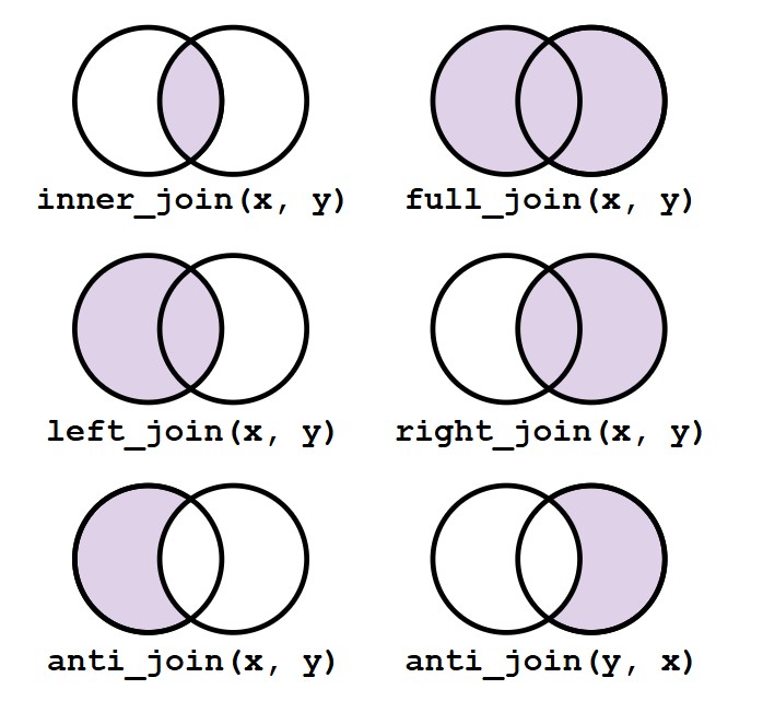
## 3 positive 867 19.2 19.4 0.0558 5.583.5 Joining Data Frames
Sometimes, we need to combine data from different sources. Here’s how to join two datasets.
# Example datasets
data_grade <- data.frame(
  subject_id = seq(1:nrow(covid)),    # subject id
  note = sample(1:20, nrow(covid), replace=TRUE)                 # Numeric
)

data_grade <- data_grade %>%
  mutate(is_graduate = ifelse(note>=10, TRUE, FALSE))

# Inner Join: Only matching subject_id rows
join_data <- full_join(covid, data_grade, by = "subject_id")

# Shown results
head(join_data)
## # A tibble: 6 × 23
## subject_id fake_first_name fake_last_name gender pan_day test_id clinic_name
## <dbl> <chr> <chr> <chr> <dbl> <chr> <chr>
## 1 1412 jhezane westerling female 4 covid inpatient …
## 2 533 penny targaryen female 7 covid clinical l…
## 3 9134 grunt rivers male 7 covid clinical l…
## 4 8518 melisandre swyft female 8 covid clinical l…
## 5 8967 SAWADOGO Laurent Benja… male 8 covid emergency …
## 6 11048 OUATTARA Siguiss… Sarah female 8 covid oncology d…
## # ℹ 16 more variables: result <chr>, demo_group <chr>, age <dbl>,
## # drive_thru_ind <dbl>, ct_result <dbl>, orderset <dbl>, payor_group <chr>,
## # patient_class <chr>, col_rec_tat <dbl>, rec_ver_tat <dbl>, age_group <chr>,
## # age_log <dbl>, age_squarred <dbl>, age_square_root <dbl>, note <int>,
## # is_graduate <lgl>3.6 Exercises 3
Try these exercises to practice dplyr functions:
Import the “blood_storage” database from the package medicaldata.
Log-transform the variable age in data and save the result as age.login the dataframe.
Arranging the dataframe using the age column.
Create a new variable called PVol.squared with values equal to the square all values in PVol (Prostate volume).
Create a new variable called PVol.squared_root with values equal to the square root all values in PVol (Prostate volume).
Compute the proportion of African American using the column AA (0 = “non‐African-American”; 1 = “African American”).
Compute the proportion of African American by Tumor volume (using the variable TVol) and the mean and variance of the column age.
Filter out the records for which (PreopPSA >= 10) and (Recurrence == 0) using the filter function.
Create a new column called subject_id and merge the “covid” database with the “blood_storage” using the newly created column.
This lesson introduces essential dplyr functions for data manipulation in R. Try the exercises and explore the dataset further! 🚀